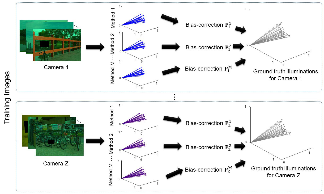
Illumination estimation is the key routine in a camera's onboard auto-white-balance (AWB) function. Illumination estimation algorithms estimate the color of the scene's illumination from an image in the form of an R,G,B vector in the sensor's raw-RGB color space. While learning-based methods have demonstrated impressive performance for illumination estimation, cameras still rely on simple statistical-based algorithms that are less accurate but capable of executing quickly on the camera's hardware. An effective strategy to improve the accuracy of these fast statistical-based algorithms is to apply a post-estimate bias correction function to transform the estimated R,G,B vector such that it lies closer to the correct solution. Recent work by Finlayson, Interface Focus, 2018 showed that a bias correction function can be formulated as a projective transform because the magnitude of the R,G,B illumination vector does not matter to the AWB procedure. This paper builds on this finding and shows that further improvements can be obtained by using an as-projective-as-possible (APAP) projective transform that locally adapts the projective transform to the input R,G,B vector. We demonstrate the effectiveness of the proposed APAP bias correction on several well-known statistical illumination estimation methods. We also describe a fast lookup method that allows the APAP transform to be performed with only a few lookup operations.
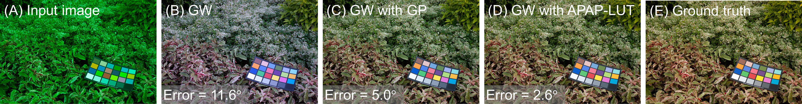
Projective bias correction of the estimated illuminant of the gray world algorithm (GW). (A) A raw Canon EOS-1Ds image from the NUS dataset. (B) The corrected image using the GW algorithm. (C) The corrected image using the global projective transformation (GP). (D) The corrected image using the as-projective-as-possible with the lookup table (APAP-LUT). (E) The ground truth image.
We applied our proposed projective bias correction transformations to four different statistical-based methods: (i) gray wrold, (ii) Gray edges, (iii) shades of gray, and (iv) distribution PCA.
* For Shades of gray, the Minkowski norm (p) was set to 4. * The first and second differentiations were used for gray edges with p=6 and σ=2. * For the distribution PCA method, the selected percentage rate was 3.5%. * All other methods source code collected from colorconstancy.com and NUS dataset webpage
Bias Correction Methods:For each illumination estimation method, we evaluate our proposed projective bias correction transformations, which are: (i) global projective transformation (GP), (ii) as-projective-as-possible bias correction (APAP), and (iii) APAP with the lookup table (APAP-LUT).
* We used σ_w=3.0 and γ=0.0625 for our APAP bias correction. The LUT consisted of 16×16 bins.
Datasets:We evaluated our method on three different datasets: (i) the NUS dataset, (ii) the reprocessed version of Gehler's dataset (Gehler-Shi dataset), and (iii) the INTEL-TUT dataset.
As there are different ground-truth illuminants available for the Gehler-Shi dataset, we recalculated the ground-truth illuminants from the color rendition chart provided in each image of the dataset.
We used three-cross-fold validation for each camera in each dataset.
We reported the mean, median, best 25%, and worst 25% performance for each method before and after our correction, where the best 25% and worst 25% are the mean of the smallest 25% error values and the mean of the highest 25% error values, respectively.
The results of gray world, gray edges, shades of gray, and distribution PCA methods may differ slightly from other reported results in the literature, because we used fixed parameters in all experiments instead of fine-tuning the parameters per camera.
| Method | Mean | Median | Best 25% | Worst 25% |
|---|---|---|---|---|
| Gray world | 4.17 | 3.15 | 0.87 | 9.23 |
| Gray edges (1st-order) | 5.08 | 3.38 | 0.90 | 12.14 |
| Gray edges (2nd-order) | 5.90 | 4.18 | 1.22 | 13.13 |
| Shades of gray | 3.28 | 2.46 | 0.76 | 7.24 |
| Distribution PCA | 4.30 | 2.95 | 0.79 | 10.05 |
| Gray world + GP | 2.64 | 1.93 | 0.64 | 5.81 |
| Gray edges (1st-order) + GP | 3.71 | 2.34 | 0.80 | 9.08 |
| Gray edges (2nd-order) + GP | 3.31 | 2.30 | 0.68 | 7.79 |
| Shades of gray + GP | 2.75 | 2.04 | 0.64 | 6.02 |
| Distribution PCA + GP | 2.90 | 2.22 | 0.68 | 6.25 |
| Gray world + APAP | 2.40 | 1.76 | 0.55 | 5.42 |
| Gray edges (1st-order) + APAP | 3.16 | 1.93 | 0.54 | 8.13 |
| Gray edges (2nd-order) + APAP | 3.01 | 1.86 | 0.56 | 7.57 |
| Shades of gray + APAP | 2.43 | 1.69 | 0.53 | 5.56 |
| Distribution PCA + APAP | 2.45 | 1.72 | 0.52 | 5.67 |
| Gray world + APAP-LUT | 2.52 | 1.83 | 0.60 | 5.62 |
| Gray edges (1st-order) + APAP-LUT | 3.11 | 2.14 | 0.63 | 7.39 |
| Gray edges (2nd-order) + APAP-LUT | 3.09 | 2.08 | 0.63 | 7.41 |
| Shades of gray + APAP-LUT | 2.55 | 1.90 | 0.57 | 5.65 |
| distribution PCA + GP | 2.59 | 1.96 | 0.59 | 5.69 |
| Method | Mean | Median | Best 25% | Worst 25% |
|---|---|---|---|---|
| Gray world | 4.90 | 3.74 | 1.04 | 10.83 |
| Gray edges (1st-order) | 5.57 | 3.52 | 0.95 | 13.61 |
| Gray edges (2nd-order) | 6.05 | 3.76 | 1.09 | 14.61 |
| Shades of gray | 3.77 | 2.32 | 0.53 | 9.39 |
| Distribution PCA | 4.17 | 2.62 | 0.53 | 10.26 |
| Gray world + GP | 3.13 | 2.40 | 0.64 | 6.89 |
| Gray edges (1st-order) + GP | 4.23 | 2.64 | 0.63 | 10.48 |
| Gray edges (2nd-order) + GP | 4.32 | 2.56 | 0.66 | 10.85 |
| Shades of gray + GP | 3.38 | 2.30 | 0.54 | 8.08 |
| Distribution PCA + GP | 3.57 | 2.32 | 0.59 | 8.53 |
| Gray world + APAP | 2.76 | 2.02 | 0.53 | 6.21 |
| Gray edges (1st-order) + APAP | 3.98 | 2.37 | 0.57 | 10.10 |
| Gray edges (2nd-order) + APAP | 4.26 | 2.48 | 0.55 | 11.05 |
| Shades of gray + APAP | 3.13 | 2.04 | 0.51 | 7.61 |
| Distribution PCA + APAP | 3.26 | 2.07 | 0.54 | 8.03 |
| Gray world + APAP-LUT | 2.96 | 2.22 | 0.59 | 6.58 |
| Gray edges (1st-order) + APAP-LUT | 4.09 | 2.40 | 0.61 | 10.29 |
| Gray edges (2nd-order) + APAP-LUT | 4.21 | 2.50 | 0.61 | 10.70 |
| Shades of gray + APAP-LUT | 3.29 | 2.20 | 0.54 | 7.88 |
| distribution PCA + APAP-LUT | 3.42 | 2.27 | 0.57 | 8.24 |
| Method | Mean | Median | Best 25% | Worst 25% |
|---|---|---|---|---|
| Gray world | 4.77 | 3.75 | 0.99 | 10.29 |
| Gray edges (1st-order) | 4.62 | 2.84 | 0.94 | 11.46 |
| Gray edges (2nd-order) | 4.82 | 2.97 | 1.03 | 11.96 |
| Shades of gray | 4.99 | 3.63 | 1.08 | 11.20 |
| Distribution PCA | 4.65 | 3.39 | 0.87 | 10.75 |
| Gray world + GP | 4.68 | 3.12 | 1.15 | 11.11 |
| Gray edges (1st-order) + GP | 3.71 | 2.34 | 0.80 | 9.08 |
| Gray edges (2nd-order) + GP | 3.10 | 2.11 | 0.74 | 7.20 |
| Shades of gray + GP | 4.37 | 2.87 | 1.04 | 10.49 |
| Distribution PCA + GP | 3.65 | 2.67 | 0.98 | 8.12 |
| Gray world + APAP | 4.30 | 2.44 | 0.69 | 11.30 |
| Gray edges (1st-order) + APAP | 3.26 | 1.54 | 0.44 | 9.15 |
| Gray edges (2nd-order) + APAP | 2.73 | 1.47 | 0.41 | 7.34 |
| Shades of gray + APAP | 3.99 | 2.14 | 0.60 | 10.82 |
| Distribution PCA + APAP | 3.16 | 1.89 | 0.52 | 8.15 |
| Gray world + APAP-LUT | 4.46 | 2.85 | 0.94 | 11.01 |
| Gray edges (1st-order) + APAP-LUT | 3.38 | 2.08 | 0.64 | 8.52 |
| Gray edges (2nd-order) + APAP-LUT | 2.87 | 1.89 | 0.59 | 6.90 |
| Shades of gray + APAP-LUT | 4.11 | 2.62 | 0.84 | 10.17 |
| distribution PCA + APAP-LUT | 3.30 | 2.41 | 0.76 | 7.48 |
This study was funded in part by the Canada First Research Excellence Fund for the Vision: Science to Applications (VISTA) programme and an NSERC Discovery Grant.